SVM One-Class Classifier For Anomaly Detection

Introduction

The One-Class Support Vector Machine (SVM) is a variant of the traditional SVM. It is specifically tailored to detect anomalies. Its primary aim is to locate instances that notably deviate from the standard. Unlike conventional Machine Learning models focused on binary or multiclass classification, the one-class SVM specializes in outlier or novelty detection within datasets. In this article, you will learn how One-Class Support Vector Machine (SVM) differs from traditional SVM. You will also learn how OC-SVM works and how to implement it. You’ll also learn about its hyperparameters. 

Learning Objectives

• To understand Anomalies
• Learn about One-class SVM
• Understand how it differs from traditional Support Vector Machine (SVM)
• Hyperparameters of OC-SVM in Sklearn
• How to detect Anomalies using OC-SVM
• Use cases of One-class SVM

Understanding Anomalies

Anomalies are observations or instances that deviate significantly from a dataset’s normal behavior. These deviations can manifest in various forms, such as outliers, noise, errors, or unexpected patterns. Anomalies are often fascinating because they may represent valuable insights. They might provide insights such as identifying fraudulent transactions, detecting equipment malfunctions, or uncovering novel phenomena. Outlier and novelty detection identify anomalies and abnormal or uncommon observations.

Also Read: An End-to-end Guide on Anomaly Detection

One Class SVM

Introduction to Support Vector Machines (SVMs)

Support Vector Machines (SVMs) are a popular supervised learning algorithm for classification and regression tasks. SVMs work by finding the optimal hyperplane that separates different classes in feature space while maximizing the margin between them. This hyperplane is based on a subset of training data points called support vectors.

One-Class SVM vs Traditional SVM

• One-class SVMs represent a variant of the traditional SVM algorithm primarily employed for outlier and novelty detection tasks. Unlike traditional SVMs, which handle binary classification tasks, One-Class SVM exclusively trains on data points from a single class, known as the target class. One-class SVM aims to learn a boundary or decision function that encapsulates the target class in feature space, effectively modeling the normal behavior of the data.

• Traditional SVMs aim to find a decision boundary that maximizes the margin between different classes, allowing for optimal classification of new data points. On the other hand, One-Class SVM seeks to find a boundary that encapsulates the target class while minimizing the risk of including outliers or novel instances outside this boundary.

• Traditional SVMs require labeled data with instances from multiple classes, making them suitable for supervised classification tasks. In contrast, a One-Class SVM allows application in scenarios where only data from the target class is available, making it well-suited for unsupervised anomaly detection and novelty detection tasks.

Learn More: One-Class Classification Using Support Vector Machines

They both differ in their soft margin formulations and the way they use them:

(Soft margin in SVM is used to allow some degree of misclassification)

One-class SVM aims to discover a hyperplane with maximum margin within the feature space by separating the mapped data from the origin. On a dataset Dn = {x1, . . . , xn} with xi ∈ X (xi is a feature) and n dimensions:

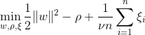
This equation represents the primal problem formulation for OC-SVM, where w is the separating hyperplane, ρ is the offset from the origin, and ξi are slack variables. They allow for a soft margin but penalize violations ξi. A hyperparameter ν ∈ (0, 1] controls the effect of the slack variable and should be adjusted according to need. The objective is to minimize the norm of w while penalizing deviations from the margin. Further, this allows a fraction of the data to fall within the margin or on the wrong side of the hyperplane.

W.X + b =0 is the decision boundary, and the slack variables penalize deviations. 

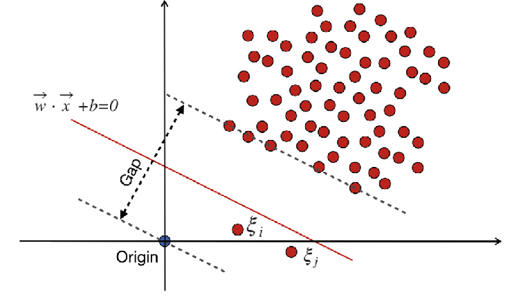
Traditional-Support Vector Machines (SVM)

Traditional-Support Vector Machines (SVM) use the soft margin formulation for misclassification errors. Or they use data points that fall within the margin or on the wrong side of the decision boundary.

Where:

w is the weight vector.

b is the bias term. 

ξi are slack variables that allow for soft margin optimization.

C is the regularization parameter that controls the trade-off between maximizing the margin and minimizing the classification error. 

ϕ(xi) represents the feature mapping function.

In traditional SVM, a supervised learning method that relies on class labels for separation incorporates slack variables to permit a certain level of misclassification. SVM’s primary objective is to separate data points of distinct classes using the decision boundary W.X + b = 0. The value of slack variables varies depending on the location of data points: they are set to 0 if the data points are located beyond the margins. If the data point resides within the margin, the slack variables range between 0 and 1, extending beyond the opposite margin if greater than 1.

Both traditional SVMs and One-Class SVMs with soft margin formulations aim to minimize the norm of the weight vector. Still, they differ in their objectives and how they handle misclassification errors or deviations from the decision boundary. Traditional SVMs optimize classification accuracy to avoid overfitting, while One-Class SVMs focus on modeling the target class and controlling the proportion of outliers or novel instances.

Also Read: The A-Z Guide to Support Vector Machine

Important Hyperparameters in One-class SVM

• nu: This is a crucial hyperparameter in One-Class SVM, which controls the proportion of outliers allowed. It sets an upper bound on the fraction of training errors and a lower bound on the fraction of support vectors. It typically ranges between 0 and 1, where lower values imply a stricter margin and may capture fewer outliers, while higher values are more permissive. The default value is 0.5.
• kernel: The kernel function determines the type of decision boundary the SVM uses. Common choices include ‘linear,’ ‘rbf’ (Gaussian radial basis function), ‘poly’ (polynomial), and ‘sigmoid.’ The ‘rbf’ kernel is often used as it can effectively capture complex non-linear relationships.
• gamma: This is a parameter for non-linear hyperplanes. It defines how much influence a single training example has. The larger the gamma value, the closer other examples must be to be affected. This parameter is specific to the RBF kernel and is typically set to ‘auto,’ which defaults to 1 / n_features.
• kernel parameters (degree, coef0): These parameters are for polynomial and sigmoid kernels. ‘degree’ is the degree of the polynomial kernel function, and ‘coef0’ is the independent term in the kernel function. Tuning these parameters might be necessary for achieving optimal performance.
• tol: This is the stopping criterion. The algorithm stops when the duality gap is smaller than the tolerance. It’s a parameter that controls the tolerance for the stopping criterion.

Working Principle of One-Class SVM

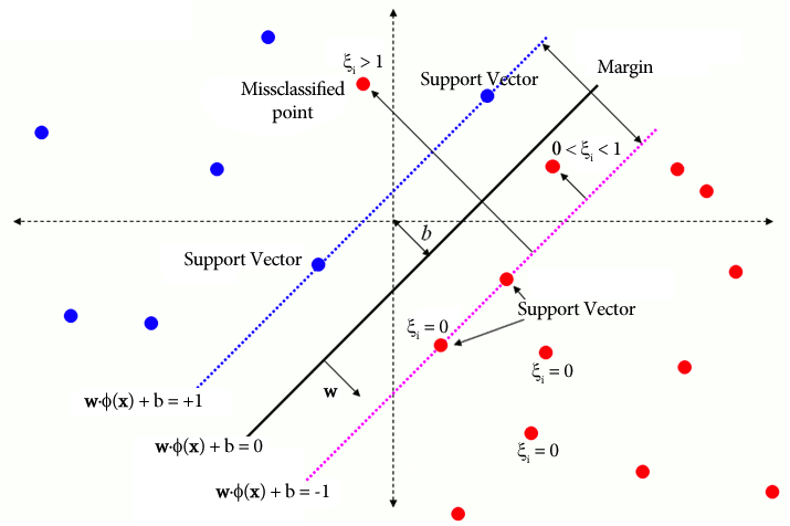
Kernel Functions in One-Class SVM

Kernel functions play a crucial role in One-Class SVM by allowing the algorithm to operate in higher-dimensional feature spaces without explicitly computing the transformations. In One-Class SVM, as in traditional SVMs, kernel functions are used to measure the similarity between pairs of data points in the input space. Common kernel functions used in One-Class SVM include Gaussian (RBF), polynomial, and sigmoid kernels. These kernels map the original input space into a higher-dimensional space, where data points become linearly separable or exhibit more distinct patterns, facilitating learning. By choosing an appropriate kernel function and tuning its parameters, One-Class SVM can effectively capture complex relationships and non-linear structures in the data, improving its ability to detect anomalies or outliers.

In cases where the data is not linearly separable, such as when dealing with complex or overlapping patterns, Support Vector Machines (SVMs) can employ a Radial Basis Function (RBF) kernel to segregate outliers from the rest of the data effectively. The RBF kernel transforms the input data into a higher-dimensional feature space that can be better separated.

Margin and Support Vectors

The concept of margin and support vectors in One-Class SVM is similar to that in traditional SVMs. The margin refers to the region between the decision boundary (hyperplane) and the nearest data points from each class. In One-Class SVM, the margin represents the region where most of the data points belonging to the target class lie. Maximizing the margin is crucial for One-Class SVM as it helps generalize new data points well and improves the model’s robustness. Support vectors are the data points that lie on or within the margin and contribute to defining the decision boundary.

In One-Class SVM, support vectors are the data points from the target class closest to the decision boundary. These support vectors play a significant role in determining the shape and orientation of the decision boundary and, thus, in the overall performance of the One-Class SVM model. By identifying the support vectors, One-Class SVM effectively learns the representation of the target class in the feature space and constructs a decision boundary that encapsulates most of the data points while minimizing the risk of including outliers or novel instances.

How Anomalies Can Be Detected Using One-Class SVM?

Detecting anomalies using One-class SVM (Support Vector Machine) through both novelty detection and outlier detection techniques:

Outlier Detection

It involves identifying observations in the training data that significantly deviate from the rest, often called outliers. Estimators for outlier detection aim to fit the areas where the training data is most concentrated, disregarding these deviant observations.

from sklearn.svm import OneClassSVM

from sklearn.datasets import load_wine

import matplotlib.pyplot as plt

import matplotlib.lines as mlines

from sklearn.inspection import DecisionBoundaryDisplay

# Load data

X = load_wine()["data"][:, [6, 9]]  # "banana"-shaped

# Define estimators (One-Class SVM)

estimators_hard_margin = {

   "Hard Margin OCSVM": OneClassSVM(nu=0.01, gamma=0.35),  # Very small nu for hard margin

}

estimators_soft_margin = {

   "Soft Margin OCSVM": OneClassSVM(nu=0.25, gamma=0.35),  # Nu between 0 and 1 for soft margin

}

# Plotting setup

fig, axs = plt.subplots(1, 2, figsize=(12, 5))

colors = ["tab:blue", "tab:orange", "tab:red"]

legend_lines = []

# Hard Margin OCSVM

ax = axs[0]

for color, (name, estimator) in zip(colors, estimators_hard_margin.items()):

   estimator.fit(X)

   DecisionBoundaryDisplay.from_estimator(

       estimator,

       X,

       response_method="decision_function",

       plot_method="contour",

       levels=[0],

       colors=color,

       ax=ax,

   )

   legend_lines.append(mlines.Line2D([], [], color=color, label=name))

ax.scatter(X[:, 0], X[:, 1], color="black")

ax.legend(handles=legend_lines, loc="upper center")

ax.set(

   xlabel="flavanoids",

   ylabel="color_intensity",

   title="Hard Margin Outlier detection (wine recognition)",

)

# Soft Margin OCSVM

ax = axs[1]

legend_lines = []

for color, (name, estimator) in zip(colors, estimators_soft_margin.items()):

   estimator.fit(X)

   DecisionBoundaryDisplay.from_estimator(

       estimator,

       X,

       response_method="decision_function",

       plot_method="contour",

       levels=[0],

       colors=color,

       ax=ax,

   )

   legend_lines.append(mlines.Line2D([], [], color=color, label=name))

ax.scatter(X[:, 0], X[:, 1], color="black")

ax.legend(handles=legend_lines, loc="upper center")

ax.set(

   xlabel="flavanoids",

   ylabel="color_intensity",

   title="Soft Margin Outlier detection (wine recognition)",

)

plt.tight_layout()

plt.show()

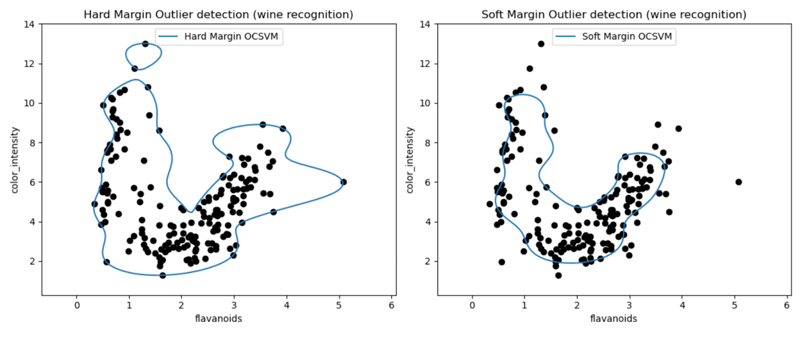
The plots allow us to visually inspect the performance of the One-Class SVM models in detecting outliers in the Wine dataset.

By comparing the results of hard margin and soft margin One-Class SVM models, we can observe how the choice of margin setting (nu parameter) affects outlier detection.

The hard margin model with a very small nu value (0.01) likely results in a more conservative decision boundary. It tightly wraps around the majority of the data points and potentially classifies fewer points as outliers.

Conversely, the soft margin model with a larger nu value (0.35) likely results in a more flexible decision boundary. Thus allowing for a wider margin and potentially capturing more outliers.

Novelty Detection

On the other hand, we apply it when the training data is free from outliers, and the goal is to determine whether a new observation is rare, i.e., very different from known observations. This latest observation here is called a novelty.

import numpy as np

from sklearn import svm

# Generate train data

np.random.seed(30)

X = 0.3 * np.random.randn(100, 2)

X_train = np.r_[X + 2, X - 2]

# Generate some regular novel observations

X = 0.3 * np.random.randn(20, 2)

X_test = np.r_[X + 2, X - 2]

# Generate some abnormal novel observations

X_outliers = np.random.uniform(low=-4, high=4, size=(20, 2))

# fit the model

clf = svm.OneClassSVM(nu=0.1, kernel="rbf", gamma=0.1)

clf.fit(X_train)

y_pred_train = clf.predict(X_train)

y_pred_test = clf.predict(X_test)

y_pred_outliers = clf.predict(X_outliers)

n_error_train = y_pred_train[y_pred_train == -1].size

n_error_test = y_pred_test[y_pred_test == -1].size

n_error_outliers = y_pred_outliers[y_pred_outliers == 1].size

import matplotlib.font_manager

import matplotlib.lines as mlines

import matplotlib.pyplot as plt

from sklearn.inspection import DecisionBoundaryDisplay

_, ax = plt.subplots()

# generate grid for the boundary display

xx, yy = np.meshgrid(np.linspace(-5, 5, 10), np.linspace(-5, 5, 10))

X = np.concatenate([xx.reshape(-1, 1), yy.reshape(-1, 1)], axis=1)

DecisionBoundaryDisplay.from_estimator(

   clf,

   X,

   response_method="decision_function",

   plot_method="contourf",

   ax=ax,

   cmap="PuBu",

)

DecisionBoundaryDisplay.from_estimator(

   clf,

   X,

   response_method="decision_function",

   plot_method="contourf",

   ax=ax,

   levels=[0, 10000],

   colors="palevioletred",

)

DecisionBoundaryDisplay.from_estimator(

   clf,

   X,

   response_method="decision_function",

   plot_method="contour",

   ax=ax,

   levels=[0],

   colors="darkred",

   linewidths=2,

)

s = 40

b1 = ax.scatter(X_train[:, 0], X_train[:, 1], c="white", s=s, edgecolors="k")

b2 = ax.scatter(X_test[:, 0], X_test[:, 1], c="blueviolet", s=s, edgecolors="k")

c = ax.scatter(X_outliers[:, 0], X_outliers[:, 1], c="gold", s=s, edgecolors="k")

plt.legend(

   [mlines.Line2D([], [], color="darkred"), b1, b2, c],

   [

       "learned frontier",

       "training observations",

       "new regular observations",

       "new abnormal observations",

   ],

   loc="upper left",

   prop=matplotlib.font_manager.FontProperties(size=11),

)

ax.set(

   xlabel=(

       f"error train: {n_error_train}/200 ; errors novel regular: {n_error_test}/40 ;"

       f" errors novel abnormal: {n_error_outliers}/40"

   ),

   title="Novelty Detection",

   xlim=(-5, 5),

   ylim=(-5, 5),

)

plt.show()

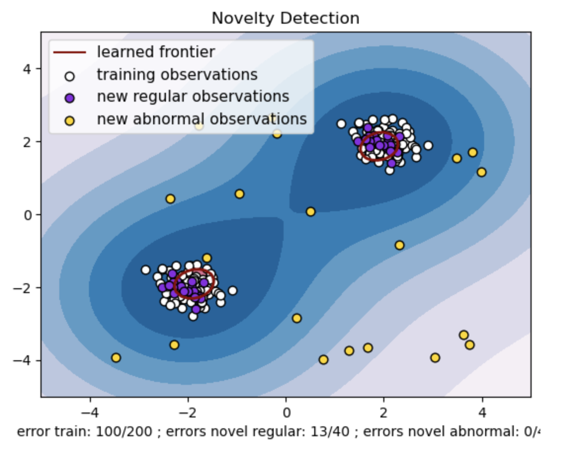
• Generate a synthetic dataset with two clusters of data points. Do this by generating them with a normal distribution around two different centers: (2, 2) and (-2, -2) for train and test data. Randomly generate twenty data points uniformly within a square region ranging from -4 to 4 along both dimensions. These data points represent abnormal observations or outliers that deviate significantly from the normal behavior observed in the train and test data.
• The learned frontier refers to the decision boundary learned by the One-class SVM model. This boundary separates the regions of the feature space where the model considers data points to be normal from the outliers.
• The color gradient from Blue to white in the contours represents the varying degrees of confidence or certainty that the One-Class SVM model assigns to different regions in the feature space, with darker shades indicating higher confidence in classifying data points as ‘normal.’ Dark Blue indicates regions with a strong indication of being ‘normal’ according to the model’s decision function. As the color becomes lighter in the contour, the model is less sure about classifying data points as ‘normal.’
• The plot visually represents how the One-class SVM model can distinguish between regular and abnormal observations. The learned decision boundary separates the regions of normal and abnormal observations. One-class SVM for novelty detection proves its effectiveness in identifying abnormal observations in a given dataset.

For nu=0.5:

The “nu” value in One-class SVM plays a crucial role in controlling the fraction of outliers tolerated by the model. It directly affects the model’s ability to identify anomalies and thus influences the prediction. We can see that the model is allowing 100 training points to be misclassified. A lower value of nu implies a stricter constraint on the allowed fraction of outliers. The choice of nu influences the model’s performance in detecting anomalies. It also requires careful tuning based on the application’s specific requirements and the dataset’s characteristics.

For gamma=0.5 and nu=0.5

In One-class SVM, the gamma hyperparameter represents the kernel coefficient for the ‘rbf’ kernel. This hyperparameter influences the shape of the decision boundary and, consequently, affects the model’s predictive performance.

When gamma is high, a single training example limits its influence to its immediate vicinity. This creates a more localized decision boundary. Therefore, data points must be closer to the support vectors to belong to the same class.

Conclusion

Utilizing One-Class SVM for anomaly detection, using outlier and novelty detection offers a robust solution across various domains. This helps in scenarios where labeled anomaly data is scarce or unavailable. Thus making it particularly valuable in real-world applications where anomalies are rare and challenging to define explicitly. Its use cases extend to diverse domains, such as cybersecurity and fault diagnosis, where anomalies have consequences. However, while One-Class SVM presents numerous benefits, it’s necessary to set the hyperparameters according to the data to get better results, which can sometimes be tedious. 

Frequently Asked Questions