How Data Efficient GANs Generate Images of Cats and Dogs?

Introduction

Generative adversarial networks are a popular framework for Image generation. In this article we’ll train Data-efficient GANs with Adaptive Discriminator Augmentation that addresses the challenge of limited training data. Adaptive Discriminator Augmentation dynamically adjusts data augmentation during GAN training, preventing discriminator overfitting and enhancing model generalization. By employing invertible augmentation techniques and probabilistic application, ADA ensures compatibility with GAN dynamics while maintaining the data distribution. This article will explore Adaptive Discriminator Augmentations transformative impact on GAN efficiency and image generation quality.

Learning Objectives

• Understand the fundamentals of Generative Adversarial Networks and their role in image generation.
• Learn how to load and preprocess data using TensorFlow for GAN training.
• Recognize the challenges posed by limited training data in GANs and the importance of addressing discriminator overfitting.
• Implement Adaptive Discriminator Augmentation (ADA) technique to enhance GAN training efficiency and improve image generation quality.
• Gain proficiency in generating images using GANs and evaluate their quality using metrics like Kernel Inception Distance (KID).
• Acquire practical skills in setting hyperparameters, loading datasets, and implementing pre-trained models like InceptionV3 within GAN training pipelines.

What are GANs?

Generative Adversarial Networks (GANs) represent a significant advancement in the realm of unsupervised learning within the domain of artificial intelligence. Comprising two distinct neural networks – a discriminator and a generator – GANs operate on the principle of adversarial training to generate synthetic data closely resembling real-world samples. The crux of their operation lies in the competitive interplay between these networks, where the generator endeavors to deceive the discriminator by producing increasingly realistic outputs from random noise inputs.

GANs are a type of data generation system that uses probabilistic models to capture patterns and structures in datasets. The adversarial component of GANs involves pitting generator outputs against authentic data, with a discriminator discerning between the two. The generator refines its output to approximate real-world data, while the discriminator evolves to distinguish more accurately. GANs use deep neural networks to train and optimize their architectures, showcasing their computational prowess and the use of AI algorithms.

Architecture of GANs

In this article we won’t look at the in-depth working of a GAN, we’ll focus on the implementation part of it. Here’s a high level overview of GANs:

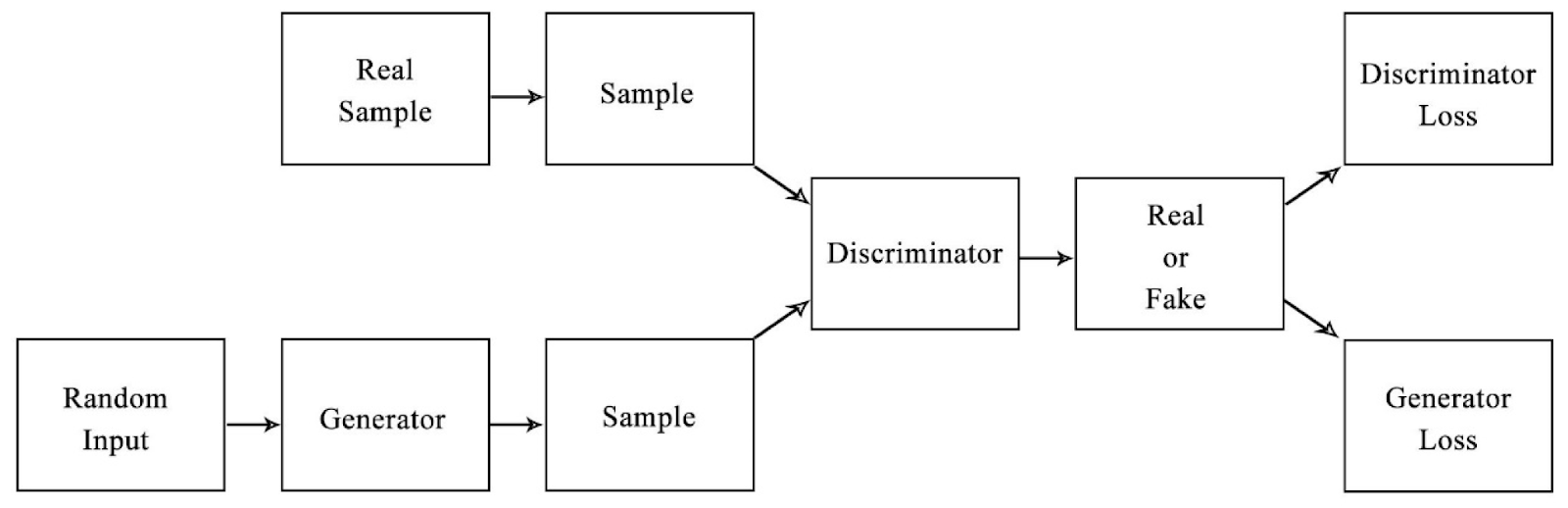
Generative Adversarial Networks consist of two main components: the Generator and the Discriminator.

• Generator Model: The generator creates realistic data from random noise, adjusting its parameters through training to mimic real samples. It’s goal is to fool the Discriminator.
• Discriminator Model: Differentiates between real and generated data, improving over time to accurately identify fake samples. Its interaction with the Generator enhances GAN’s ability to produce realistic data.

What is Data Efficient GANs?

Data Efficient GANs with Adaptive Discriminator Augmentation improves GAN training addresses discriminator overfitting due to limited data. Traditional GANs struggle with limited data, as the generator might not receive useful feedback from the discriminator. Here we’ll use adaptive data augmentation for the discriminator, ensuring it doesn’t overfit. This augmentation is applied in a differentiable and GPU-compatible manner, crucial for GAN training. Additionally, invertible data augmentation prevents “leaky augmentations” by applying transformations with some probability, preserving the original data distribution and improving discriminator regularization.

Generating Images Using GAN

In this article we’ll be working with “cats_vs_dogs” dataset from tensorflow, if you choose to work with other datasets from tensorflow you can look at the available datasets using “tfds.list_builders()”.

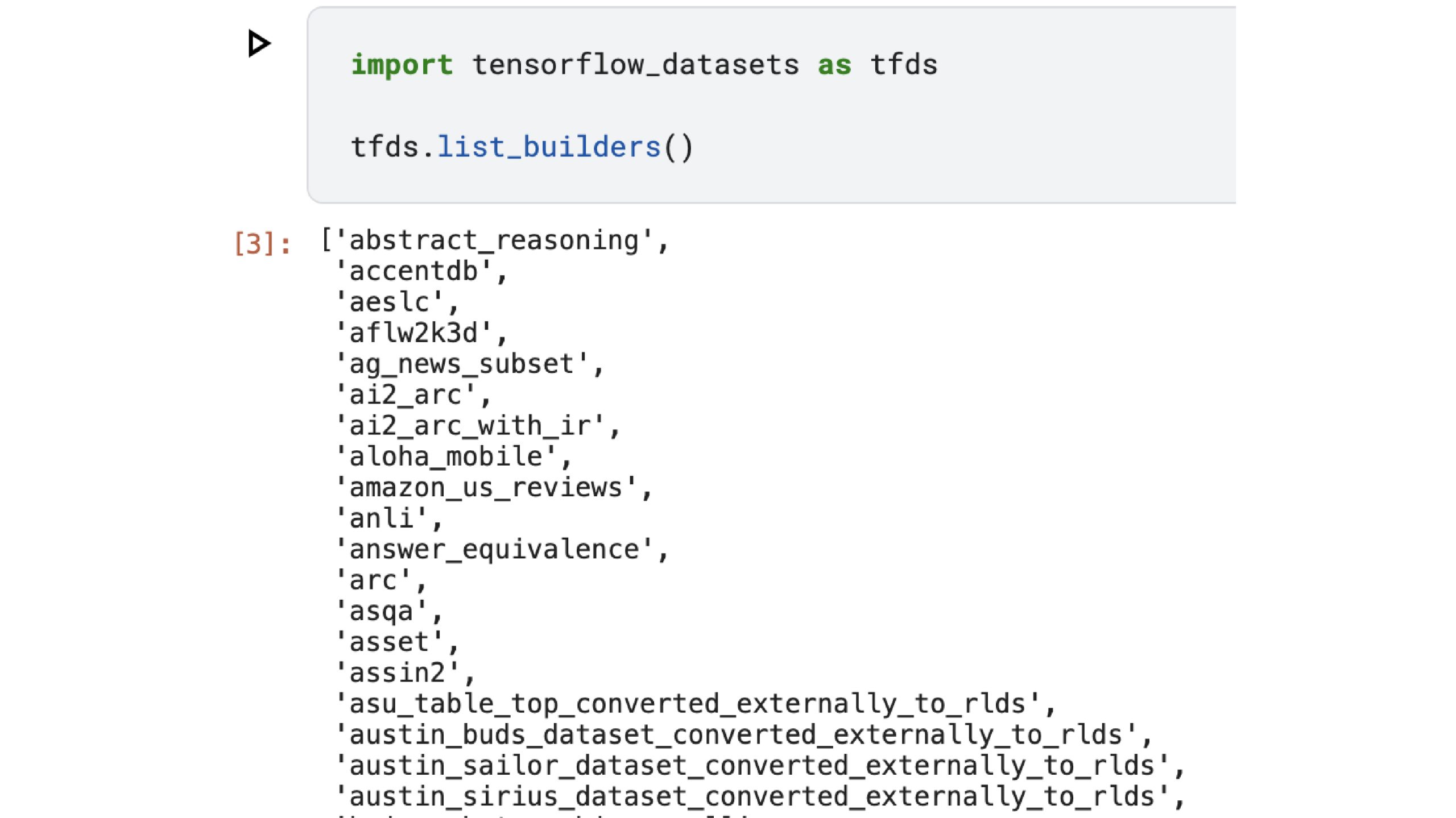
You can see more about Cats_vs_Dogs dataset here.

Step1: Import the Necessary Modules

Let’s start by loading the data, but before that let’s do some necessary imports. 

import matplotlib.pyplot as plt
import tensorflow as tf
import tensorflow_datasets as tfds
from tensorflow import keras
from keras import layers

Note: It is recommended to update your tensorflow and tensorflow-datasets before we start:

Step2: Loading the Dataset

!pip install --upgrade tensorflow
!pip install --upgrade tensorflow-datasets
Setting Hyperparameters
num_epochs = 500
image_size = 64
dataset_name = "cats_vs_dogs" 
kid_image_size = 75
padding = 0.25
# adaptive discriminator augmentation
max_translation = 0.125
max_rotation = 0.125
max_zoom = 0.25
target_accuracy = 0.85
integration_steps = 1000
# architecture
noise_size = 64
depth = 4
width = 128
leaky_relu_slope = 0.2
dropout_rate = 0.4
# optimization
batch_size = 128
learning_rate = 2e-4
beta_1 = 0.5  
ema = 0.99
Loading the data 
def round_to_int(float_value):
    return tf.cast(tf.math.round(float_value), dtype=tf.int32)

def preprocess_image(data):
    # Resize and normalize images
    image = tf.image.resize(data['image'], [image_size, image_size])
    image = tf.cast(image, tf.float32) / 255.0
    return image
def prepare_dataset(split):
    # Load dataset, preprocess images, and apply shuffling and batching
    return (
        tfds.load(dataset_name, split="train", shuffle_files=True)
        .map(preprocess_image, num_parallel_calls=tf.data.AUTOTUNE)
        .cache()
        .shuffle(10 * batch_size)
        .batch(batch_size, drop_remainder=True)
        .prefetch(buffer_size=tf.data.AUTOTUNE)
    )
train_dataset = prepare_dataset("train")
val_dataset = train_dataset
Let’s look at the images:
import matplotlib.pyplot as plt
def show_images(dataset, num_images=5):
    plt.figure(figsize=(10, 10))
    for images in dataset.take(1):
        for i in range(num_images):
            ax = plt.subplot(1, num_images, i + 1)
            plt.imshow(images[i])
            plt.axis("off")
# Display images from train and validation dataset
show_images(train_dataset)
show_images(val_dataset)
plt.show()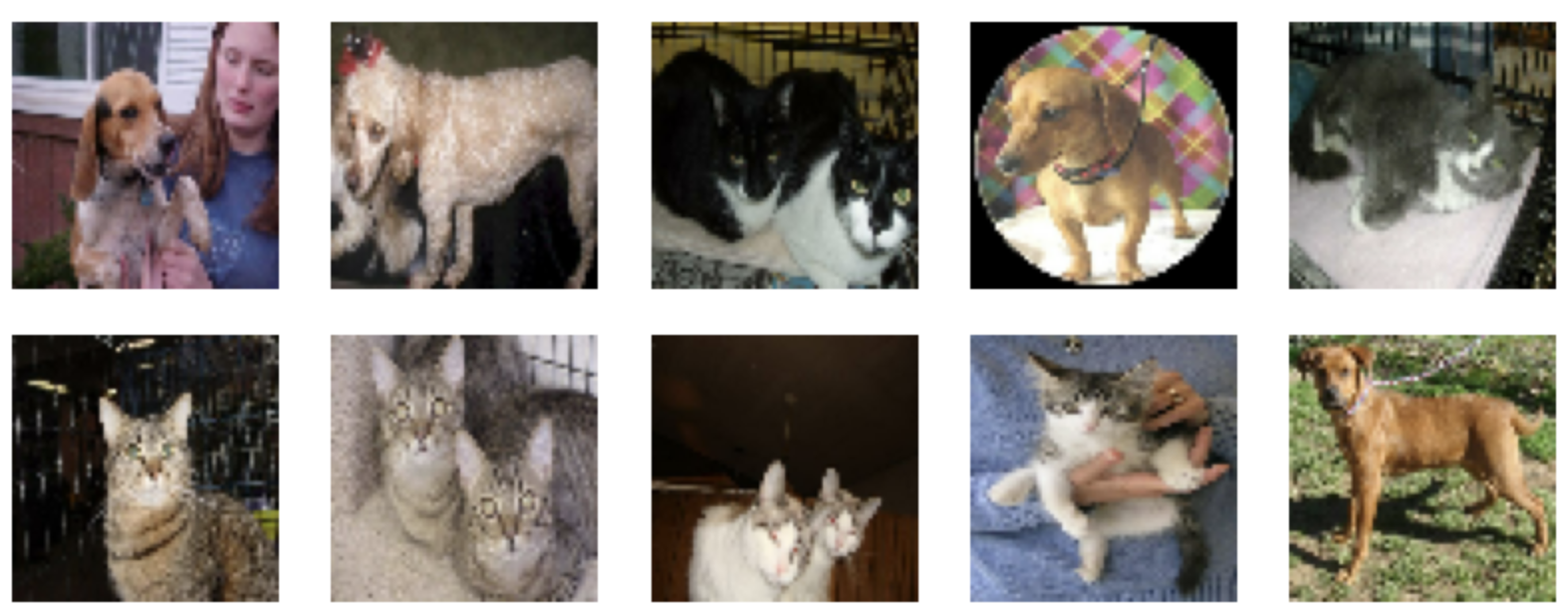

Step3: Using Pre-trained Model

We’ll be using a pre-trained InceptionV3 model along with the GAN, but we won’t be using the classification layer of the InceptionV3.

Kernel Inception Distance (KID) measures image generation quality based on differences in InceptionV3 network representations. It’s computationally efficient and unbiased, suitable for small datasets, estimating per-batch and averaging across batches.

class KID(keras.metrics.Metric):
   def __init__(self, name="kid", **kwargs):
       super().__init__(name=name, **kwargs)
       # KID is estimated per batch and is averaged across batches
       self.kid_tracker = keras.metrics.Mean()
       # Using a pretrained InceptionV3 is used without the classification layer
       self.encoder = keras.Sequential(
           [
               layers.InputLayer(input_shape=(image_size, image_size, 3)),
               layers.Rescaling(255.0),
               layers.Resizing(height=kid_image_size, width=kid_image_size),
               layers.Lambda(keras.applications.inception_v3.preprocess_input),
               keras.applications.InceptionV3(
                   include_top=False,
                   input_shape=(kid_image_size, kid_image_size, 3),
                   weights="imagenet",
               ),
               layers.GlobalAveragePooling2D(),
           ],
           name="inception_encoder",
       )
   def polynomial_kernel(self, features_1, features_2):
       feature_dimensions = tf.cast(tf.shape(features_1)[1], dtype=tf.float32)
      return (features_1 @ tf.transpose(features_2) / feature_dimensions + 1.0) ** 3.0
   def update_state(self, real_images, generated_images, sample_weight=None):
       real_features = self.encoder(real_images, training=False)
       generated_features = self.encoder(generated_images, training=False)
       # compute polynomial kernels using the two sets of features
       kernel_real = self.polynomial_kernel(real_features, real_features)
       kernel_generated = self.polynomial_kernel(
           generated_features, generated_features

       )

       kernel_cross = self.polynomial_kernel(real_features, generated_features)
       # estimate the squared maximum mean discrepancy using the average kernel values
       batch_size = tf.shape(real_features)[0]

       batch_size_f = tf.cast(batch_size, dtype=tf.float32)
      mean_kernel_real = tf.reduce_sum(kernel_real * (1.0 - tf.eye(batch_size))) / (
           batch_size_f * (batch_size_f - 1.0)
       )
       mean_kernel_generated = tf.reduce_sum(
           kernel_generated * (1.0 - tf.eye(batch_size))
       ) / (batch_size_f * (batch_size_f - 1.0))
       mean_kernel_cross = tf.reduce_mean(kernel_cross)
       kid = mean_kernel_real + mean_kernel_generated - 2.0 * mean_kernel_cross
       # update the average KID estimate
       self.kid_tracker.update_state(kid)

   def result(self):
       return self.kid_tracker.result()

   def reset_state(self):
       self.kid_tracker.reset_state()

Step4: Augmenter, Discriminator and Generator

Adaptive discriminator augmentation used here adjusts augmentation probability during training via integral control to maintain discriminator accuracy on real images near a target value.

# "hard sigmoid", useful for binary accuracy calculation from logits
def step(values):
   # negative values -> 0.0, positive values -> 1.0
   return 0.5 * (1.0 + tf.sign(values))
# augments images with a probability that is dynamically updated during training
class AdaptiveAugmenter(keras.Model):
   def __init__(self):
       super().__init__()
       # stores the current probability of an image being augmented
       self.probability = tf.Variable(0.0)
       # the corresponding augmentation names from the paper are shown above each layer
       # the authors show (see figure 4), that the blitting and geometric augmentations
       # are the most helpful in the low-data regime
       self.augmenter = keras.Sequential(
           [
               layers.InputLayer(input_shape=(image_size, image_size, 3)),
               # blitting/x-flip:
               layers.RandomFlip("horizontal"),
               # blitting/integer translation:
               layers.RandomTranslation(
                   height_factor=max_translation,
                   width_factor=max_translation,
                   interpolation="nearest",
               ),
               # geometric/rotation:
               layers.RandomRotation(factor=max_rotation),
               # geometric/isotropic and anisotropic scaling:
               layers.RandomZoom(
                   height_factor=(-max_zoom, 0.0), width_factor=(-max_zoom, 0.0)
               ),
           ],
           name="adaptive_augmenter",
       )
   def call(self, images, training):
       if training:
           augmented_images = self.augmenter(images, training)
           # during training either the original or the augmented images are selected
           # based on self.probability
           augmentation_values = tf.random.uniform(
               shape=(batch_size, 1, 1, 1), minval=0.0, maxval=1.0
           )
           augmentation_bools = tf.math.less(augmentation_values, self.probability)
           images = tf.where(augmentation_bools, augmented_images, images)
       return images
   def update(self, real_logits):
       current_accuracy = tf.reduce_mean(step(real_logits))
       # the augmentation probability is updated based on the discriminator's
       # accuracy on real images
       accuracy_error = current_accuracy - target_accuracy
       self.probability.assign(
           tf.clip_by_value(
               self.probability + accuracy_error / integration_steps, 0.0, 1.0
           )
       )
We’ll be using the tried and tested Deeply connected GAN’s (DC-GAN) generator and discriminator. 

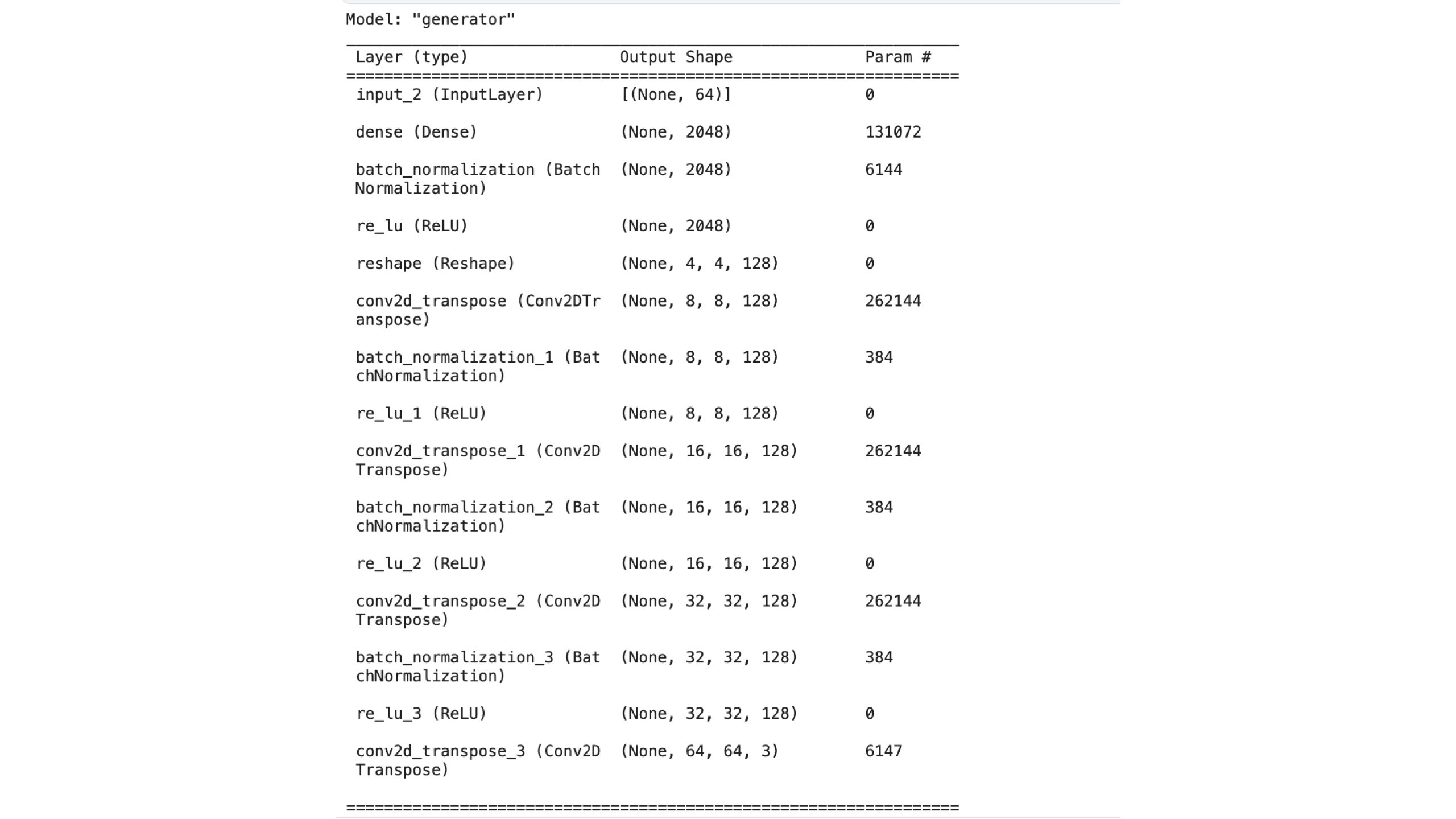
def get_generator():
   noise_input = keras.Input(shape=(noise_size,))
   x = layers.Dense(4 * 4 * width, use_bias=False)(noise_input)
   x = layers.BatchNormalization(scale=False)(x)
   x = layers.ReLU()(x)
   x = layers.Reshape(target_shape=(4, 4, width))(x)
   for _ in range(depth - 1):
       x = layers.Conv2DTranspose(
           width, kernel_size=4, strides=2, padding="same", use_bias=False,
       )(x)
       x = layers.BatchNormalization(scale=False)(x)
       x = layers.ReLU()(x)
   image_output = layers.Conv2DTranspose(
       3, kernel_size=4, strides=2, padding="same", activation="sigmoid",
   )(x)
   return keras.Model(noise_input, image_output, name="generator")
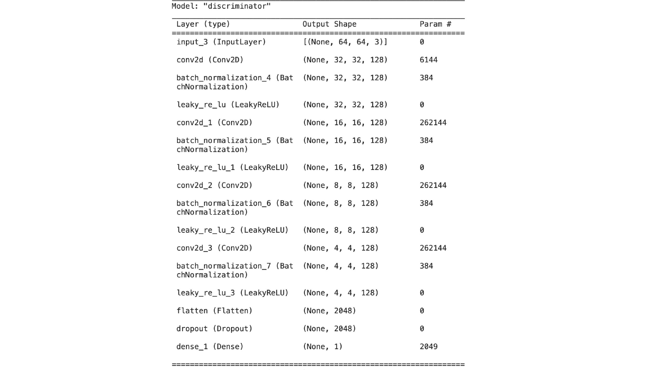
# DCGAN discriminator
def get_discriminator():
   image_input = keras.Input(shape=(image_size, image_size, 3))
   x = image_input
   for _ in range(depth):
       x = layers.Conv2D(
           width, kernel_size=4, strides=2, padding="same", use_bias=False,
       )(x)
       x = layers.BatchNormalization(scale=False)(x)
       x = layers.LeakyReLU(alpha=leaky_relu_slope)(x)
   x = layers.Flatten()(x)
   x = layers.Dropout(dropout_rate)(x)
   output_score = layers.Dense(1)(x)
   return keras.Model(image_input, output_score, name="discriminator")
class GAN_ADA(keras.Model):
   def __init__(self):
       super().__init__()
       self.augmenter = AdaptiveAugmenter()
       self.generator = get_generator()
       self.ema_generator = keras.models.clone_model(self.generator)
       self.discriminator = get_discriminator()
       self.generator.summary()
       self.discriminator.summary()
   def compile(self, generator_optimizer, discriminator_optimizer, **kwargs):
       super().compile(**kwargs)
       # separate optimizers for the two networks
       self.generator_optimizer = generator_optimizer
       self.discriminator_optimizer = discriminator_optimizer
       self.generator_loss_tracker = keras.metrics.Mean(name="g_loss")
       self.discriminator_loss_tracker = keras.metrics.Mean(name="d_loss")
       self.real_accuracy = keras.metrics.BinaryAccuracy(name="real_acc")
       self.generated_accuracy = keras.metrics.BinaryAccuracy(name="gen_acc")
       self.augmentation_probability_tracker = keras.metrics.Mean(name="aug_p")
       self.kid = KID()
   @property
   def metrics(self):
       return [
           self.generator_loss_tracker,
           self.discriminator_loss_tracker,
           self.real_accuracy,
           self.generated_accuracy,
          self.augmentation_probability_tracker,
           self.kid,
       ]
   def generate(self, batch_size, training):
       latent_samples = tf.random.normal(shape=(batch_size, noise_size))
       # use ema_generator during inference
       if training:
           generated_images = self.generator(latent_samples, training)
       else:
           generated_images = self.ema_generator(latent_samples, training)

       return generated_images
   def adversarial_loss(self, real_logits, generated_logits):
       # this is usually called the non-saturating GAN loss
       real_labels = tf.ones(shape=(batch_size, 1))
       generated_labels = tf.zeros(shape=(batch_size, 1))
      # the generator tries to produce images that the discriminator considers as real
       generator_loss = keras.losses.binary_crossentropy(
           real_labels, generated_logits, from_logits=True
       )
       # the discriminator tries to determine if images are real or generated
       discriminator_loss = keras.losses.binary_crossentropy(
           tf.concat([real_labels, generated_labels], axis=0),
           tf.concat([real_logits, generated_logits], axis=0),
           from_logits=True,
       )
       return tf.reduce_mean(generator_loss), tf.reduce_mean(discriminator_loss)
   def train_step(self, real_images):
       real_images = self.augmenter(real_images, training=True)
       # use persistent gradient tape because gradients will be calculated twice
       with tf.GradientTape(persistent=True) as tape:
           generated_images = self.generate(batch_size, training=True)
           # gradient is calculated through the image augmentation
           generated_images = self.augmenter(generated_images, training=True)
           # separate forward passes for the real and generated images, meaning
           # that batch normalization is applied separately
           real_logits = self.discriminator(real_images, training=True)
           generated_logits = self.discriminator(generated_images, training=True)
           generator_loss, discriminator_loss = self.adversarial_loss(
               real_logits, generated_logits
           )
       # calculate gradients and update weights
       generator_gradients = tape.gradient(
           generator_loss, self.generator.trainable_weights
       )
       discriminator_gradients = tape.gradient(
           discriminator_loss, self.discriminator.trainable_weights
       )
       self.generator_optimizer.apply_gradients(
           zip(generator_gradients, self.generator.trainable_weights)
       )
       self.discriminator_optimizer.apply_gradients(
           zip(discriminator_gradients, self.discriminator.trainable_weights)
       )
       # update the augmentation probability based on the discriminator's performance
       self.augmenter.update(real_logits)
       self.generator_loss_tracker.update_state(generator_loss)
       self.discriminator_loss_tracker.update_state(discriminator_loss)
       self.real_accuracy.update_state(1.0, step(real_logits))
       self.generated_accuracy.update_state(0.0, step(generated_logits))
      self.augmentation_probability_tracker.update_state(self.augmenter.probability)
       # track the exponential moving average of the generator's weights to decrease
       # variance in the generation quality
       for weight, ema_weight in zip(
           self.generator.weights, self.ema_generator.weights
       ):
           ema_weight.assign(ema * ema_weight + (1 - ema) * weight)
       # KID is not measured during the training phase for computational efficiency

       return {m.name: m.result() for m in self.metrics[:-1]}
   def test_step(self, real_images):
       generated_images = self.generate(batch_size, training=False)
       self.kid.update_state(real_images, generated_images)
       # 0nly KID is measured during the evaluation phase for computational efficiency
       return {self.kid.name: self.kid.result()}
   def plot_images(self, epoch=None, logs=None, num_rows=3, num_cols=6, interval=5):
       # plot random generated images for visual evaluation of generation quality
       if epoch is None or (epoch + 1) % interval == 0:
           num_images = num_rows * num_cols
           generated_images = self.generate(num_images, training=False)
           plt.figure(figsize=(num_cols * 2.0, num_rows * 2.0))
           for row in range(num_rows):
               for col in range(num_cols):
                   index = row * num_cols + col
                   plt.subplot(num_rows, num_cols, index + 1)
                   plt.imshow(generated_images[index])
                   plt.axis("off")
           plt.tight_layout()
           plt.show()
           plt.close()

Step5: Training the Model

Make sure to adjust augmentation probability based on real accuracy. Healthy GAN training maintains discriminator accuracy between 80-95%

# create and compile the model
model = GAN_ADA()
model.compile(
   generator_optimizer=keras.optimizers.Adam(learning_rate, beta_1),
   discriminator_optimizer=keras.optimizers.Adam(learning_rate, beta_1),
)
# save the best model based on the validation KID metric
checkpoint_path = "gan_model"
checkpoint_callback = tf.keras.callbacks.ModelCheckpoint(
   filepath=checkpoint_path,
   save_weights_only=True,
   monitor="val_kid",
   mode="min",
   save_best_only=True,
)
# run training and plot generated images periodically
model.fit(
   train_dataset,
   epochs=num_epochs,
   validation_data=val_dataset,
   callbacks=[
       keras.callbacks.LambdaCallback(on_epoch_end=model.plot_images),
       checkpoint_callback,
   ],
)

Model Architecture

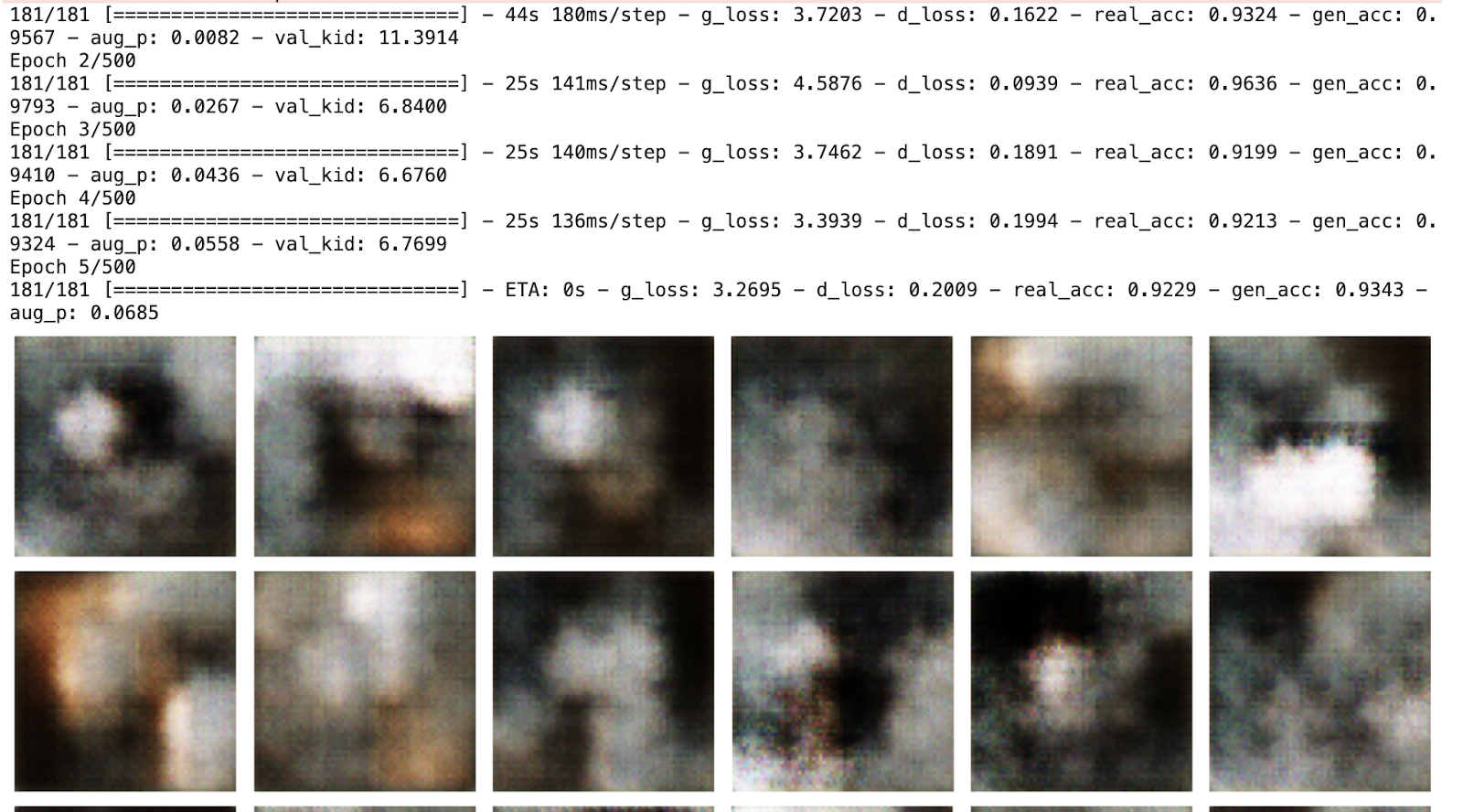
Generated images

I have trained the model for 500 epochs, with the random noise model starts generating these images at the 5th epoch

After 500 epochs the images this is the result: 

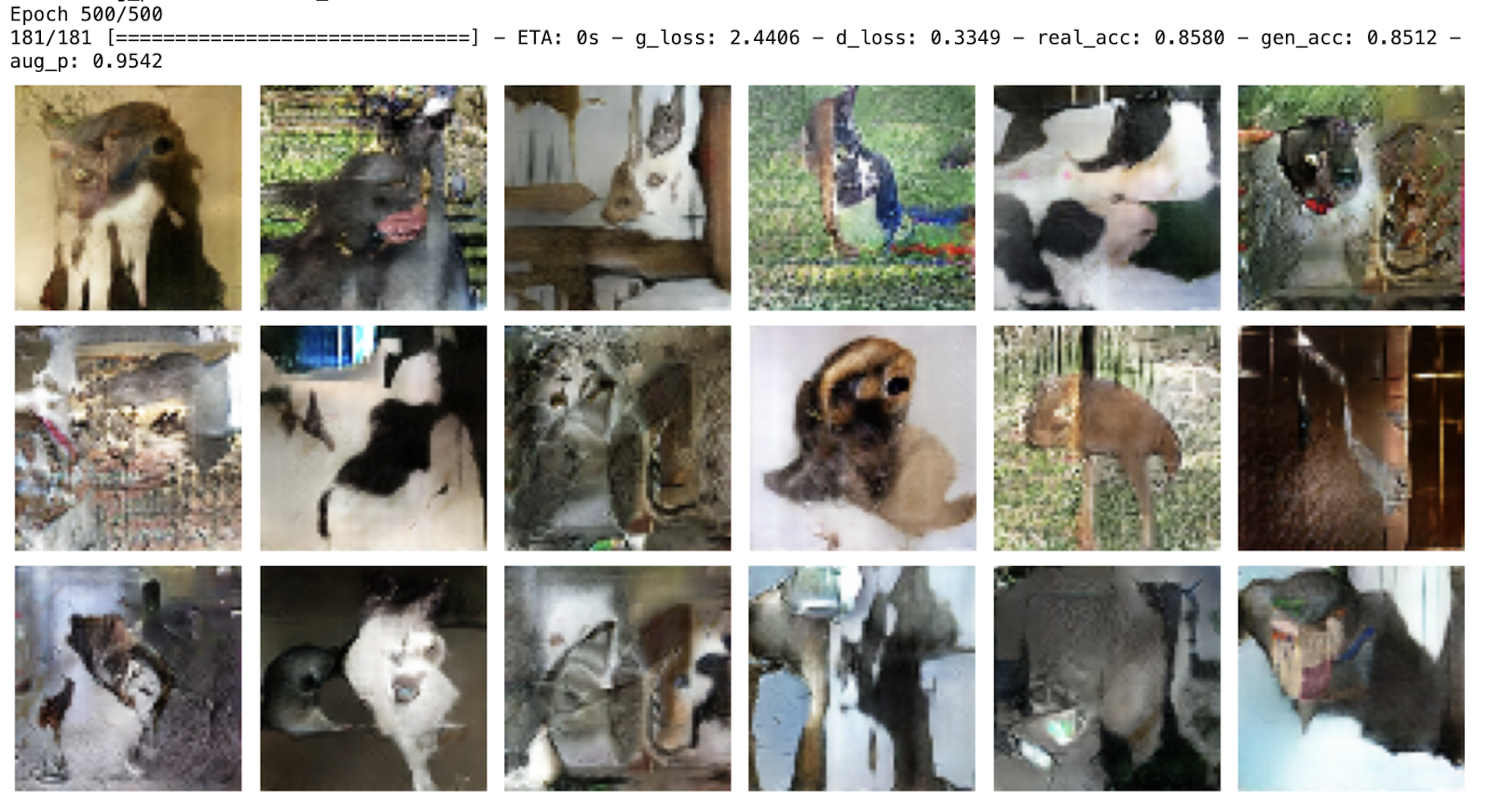
The model should be trained for at least 6000 epochs before we might start seeing clear images of cats and dogs. 

Conclusion

Balancing simplicity and quality in GAN implementation involves critical considerations. I recommend you choose an appropriate resolution, choose the right number of epochs for your use case, and careful handling of upsampling. You can also use Spectral normalization and dropout layers to enhance stability and quality. GANs are difficult to deal with, they need lots of tuning and they take a lot of time for training. Explore newer GANs for better image generation or you can look at other probabilistic techniques too. 

Key Takeaways

• Gained insights on the importance of Image Augmentation.
• Learn about Generators and Discriminators of GANs and how to generate new images.
• Kernel Inception Distance (KID) is a metric used to evaluate the quality of generated images based on differences in InceptionV3 network representations.
• GAN architecture consists of two main components: the generator and the discriminator, which work adversarially to generate realistic data.
• We Learned and explored to use Data Loaders efficiently.
• Explored and learned to work with GANs and train them.
• TensorFlow provides robust tools and libraries for implementing GANs for image generation, including loading datasets, defining models, and training pipelines.

Frequently Asked Questions